A radioligand is a radioactively labeled drug that can associate with a receptor, transporter, enzyme, or any protein of interest. Measuring the rate and extent of binding provides information on the number of binding sites, and their affinity and accessibility for various drugs. Radioligand binding experiments are easy to perform, and provide useful data in many fields. But many find it difficult to analyze radioligand binding data. That's why I wrote this booklet.

If you want more detailed information beyond the scope of this booklet, consult one of these general references:

• LE Limbird, Cell surface receptors: A short course on theory and methods, Kluwer Academic Publishers, second edition, 1996.
• HI Yamamura, et. al. Methods in neurotransmitter receptor analysis, Raven Press, 1990.
• T Kenakin, Pharmacologic analysis of drug-receptor interaction, second edition, Raven Press, 1993.

You have permission to duplicate this booklet for use in teaching and research, provided that you duplicate the entire document (including the copyright page) and don't charge for copies. You may also download this document from the internet (http://www.graphpad.com) or order additional copies from GraphPad Software.

I thank Drs. Lee Limbird and Richard Neubig for making very helpful comments!

The law of mass action

Most analyses of radioligand binding experiments are based on a simple model, called the law of mass action:

The model is based on these simple ideas:

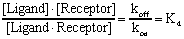
At equilibrium, ligandreceptor complexes form at the same rate that they dissociate:

Rearrange to define the equilibrium dissociation constant K_d.

The K_d, expressed in units of moles/liter or molar, is the concentration of ligand which occupies half of the receptors at equilibrium. A small K_d means that the receptor has a high affinity for the ligand. A large K_d means that the receptor has a low affinity for the ligand. Don't mix up K_d, the equilibrium dissociation constant, with k_off, the dissociation rate constant. They are not the same, and aren't even expressed in the same units.

The law of mass action predicts the fractional receptor occupancy at equilibrium as a function of ligand concentration. Fractional occupancy is the fraction of all receptors that are bound to ligand.

A bit of algebra creates a useful equation. Multiply both numerator and denominator by [Ligand] and divide both by [LigandReceptor]. Then substitute the definition of K_d.

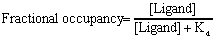
When [Ligand]=0, the occupancy equals zero. When [Ligand] is very high (many times K_d) , the fractional occupancy approaches 1.00. When [Ligand]=K_d, fractional occupancy is 0.50. The approach to saturation as [ligand] increases is slower than many people appreciate. When the ligand concentration equals four times its K_d, it will only occupy 80% of the receptors at equilibrium. The occupancy rises to 90% when the ligand concentration equals 9 times the K_d. It takes a concentration equal to 99 times the K_d to occupy 99% of the receptors at equilibrium.

Assumptions inherent in the law of mass action

Although termed a "law", the law of mass action is simply a model based on these assumptions:

If these assumptions are not met, you have two choices. One choice is to develop a more complicated model, beyond the scope of this booklet. The other choice is to analyze your data in the usual way, but interpret the results as an empirical description of the data without attributing rigorous thermodynamic meaning to the K_d values and rate constants.

Saturation binding experiments

Saturation binding experiments measure specific binding at equilibrium at various concentrations (often 6-12) of the radioligand to determine receptor number and affinity. Because this kind of experiment can be graphed as a Scatchard plot (more accurately attributed to Rosenthal), they are sometimes called "Scatchard experiments".

The analyses depend on the assumption that the incubation has reached equilibrium. This can take anywhere from a few minutes to many hours, depending on the ligand, receptor, temperature, and other experimental conditions. Since lower concentrations of radioligand take longer to equilibrate, use a low concentration of radioligand (perhaps 10-20% of the Kd) when measuring how long it takes the incubation to reach equilibrium.

Nonspecific binding

In addition to binding to the receptors of physiological interest, radioligands bind to nonreceptor sites. When performing radioligand binding experiments, you need to measure both total and nonspecific binding, and calculate specific (receptor) binding as the difference.

Assess nonspecific binding by measuring radioligand binding in the presence of a concentration of an unlabeled compound that binds to essentially all the receptors. Since all the receptors are occupied by the unlabeled drug, the radioligand only binds nonspecifically.

Which unlabeled drug should you use? The obvious answer is to use the same compound as the radioligand, but unlabeled. In many cases, this is necessary as no other drug is known to bind to the receptors. But most investigators avoid using the same compound as the hot and cold ligand for routine work, and prefer to define nonspecific binding with a standard drug that is known to bind to that particular receptor.

What concentration of unlabeled drug should you use? You want to use enough to block virtually all the specific radioligand binding, but not so much that you cause more general physical changes to the membrane that might alter specific binding. If you are studying a well-characterized receptor, a useful rule-of-thumb is to use the unlabeled compound at a concentration equal to 100 times its K_d for the receptors.

Ideally, you should get the same results defining nonspecific binding with a range of concentrations of several drugs.

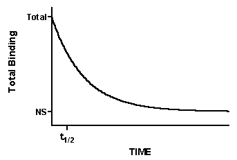
Nonspecific binding is generally proportional to the concentration of radioligand (within the range it is used). The left figure shows total and nonspecific binding. The dotted curve shows the difference between total and nonspecific binding - the specific binding.

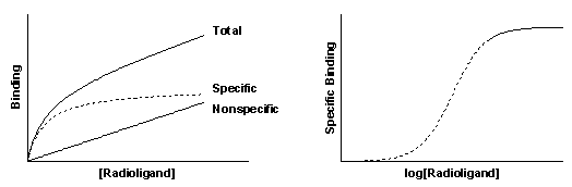
The right panel shows the specific binding again on a graph with a logarithmic X axis. Notice that the saturation binding curve plotted on a log axis looks like the familiar sigmoidal dose-response curve. The dotted curves in the two panels represent the same range of radioligand concentrations. The solid portion of the curve on the right shows binding at higher radioligand concentrations. These high concentrations are rarely used because radioligands are expensive and nonspecific binding would be too high a fraction of total binding.

Fitting a curve to determine B_max and K_d

Equilibrium specific binding at a particular radioligand concentration equals fractional occupancy times the total receptor number (Bmax):

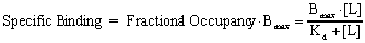
This equation describes a rectangular hyperbola or a binding isotherm. [L] is the concentration of free radioligand, the value plotted on the X axis. Bmax is the total number of receptors expressed in the same units as the Y values (i.e., cpm, sites/cell or fmol/mg protein) and Kd is the equilibrium dissociation constant (expressed in the same units as [L], usually nM). Typical values might be a Bmax of 10-1000 fmol binding sites per milligram of protein and a Kd between 10 pM and 100 nM.

To determine the B_max and K_d, fit data to the equation using nonlinear regression.

This analysis is based on these assumptions:

• Binding follows the law of mass action and has equilibrated.
• There is only one population of receptors.

Scatchard plots

Before nonlinear regression programs were widely available, scientists transformed data to make a linear graph, and then analyzed the transformed data with linear regression. There are several ways to linearize binding data, but Scatchard plots (more accurately attributed to Rosenthal) are used most often. In this plot, the X axis is specific binding (usually labeled "bound") and the Y axis is the ratio of specific binding to concentration of free radioligand (usually labeled "bound/free"). Bmax is the X intercept; Kd is the negative reciprocal of the slope.

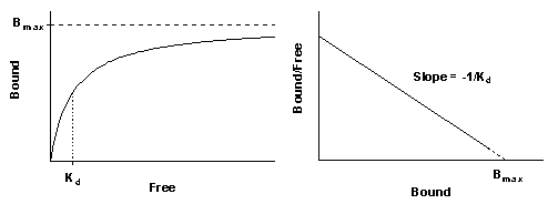
When making a Scatchard plot, you have to choose units for the Y axis. One choice is to express both free ligand and specific binding in cpm so the ratio bound/free is a unitless fraction. The advantage of this choice is that you can interpret Y values as the fraction of radioligand bound to receptors. If the highest Y value is large (greater than 0.10), then the free concentration will be substantially less than the added concentration of radioligand, and the standard analyses won't work. You should either revise your experimental protocol or use special analysis methods that deal with ligand depletion (see page 29). The disadvantage is that you cannot interpret the slope of the line without performing unit conversions.

An alternative is to express the Y axis as sites/cell/nM or fmol/mg/nM. While these values are hard to interpret, they simplify calculation of the K_d which equals the reciprocal of the slope. The specific binding units cancel when you calculate the slope. The negative reciprocal of the slope is expressed in units of concentration (nM) which equals the K_d.

Why you shouldn't analyze data with Scatchard plots

While Scatchard plots are very useful for visualizing data, they are not the most accurate way to analyze data. The problem is that the linear transformation distorts the experimental error. Linear regression assumes that the scatter of points around the line follows a Gaussian distribution and that the standard deviation is the same at every value of X. These assumptions are not true with the transformed data. A second problem is that the Scatchard transformation alters the relationship between X and Y. The value of X (bound) is used to calculate Y (bound/free), and this violates the assumptions of linear regression.

Since the assumptions of linear regression are violated, the B_max and K_d you determine by linear regression of Scatchard transformed data are likely to be further from their true values than the B_max and K_d determined by nonlinear regression. Considering all the time and effort you put into collecting data, you want to use the best possible analysis technique. Nonlinear regression produces the most accurate results. Scatchard plots produce approximate results.

The figure below shows the problem of transforming data. The left panel shows data that follows a rectangular hyperbola (binding isotherm). The right panel is a Scatchard plot of the same data. The solid curve on the left was determined by nonlinear regression. The solid line on the right shows how that same curve would look after a Scatchard transformation. The dotted line shows the linear regression fit of the transformed data. The transformation amplified and distorted the scatter, and thus the linear regression fit does not yield the most accurate values for B_max and K_d. In this example, the B_max determined by the Scatchard plot is about 25% too large and the K_d determined by the Scatchard plot is too high. The errors could just as easily have gone in the other direction.

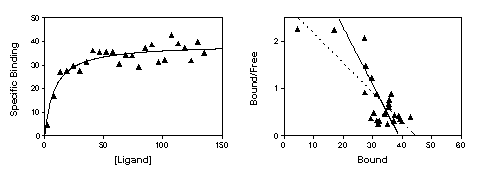
The experiment in the figure was designed to determine the B_max and the experimenter didn't care too much about the value of the K_d. So it was appropriate to obtain only a few data points at the beginning of the curve and many in the plateau region. Note however how the Scatchard transformation gives undo weight to the data point collected at the lowest concentration of radioligand (the lower left point in the left panel, the upper left point in the right panel). This point dominates the linear regression calculations on the Scatchard graph. It has "pulled" the regression line to become shallower, resulting in an overestimate of the B_max.

Although it is inappropriate to analyze data by performing linear regression on a Scatchard plot, it is often helpful to display data as a Scatchard plot. Many people find it easier to visually interpret Scatchard plots than binding curves, especially when comparing results from different experimental treatments.

Competitive binding experiments

What is a competitive binding curve?

Competitive binding experiments measure the binding of a single concentration of labeled ligand in the presence of various concentrations of unlabeled ligand.

Competitive binding experiments are used to:

Performing the experiment

The experiment is done with a single concentration of radioligand. How much should you use? There is no clear answer. Higher concentrations of radioligand are more expensive and result in higher nonspecific binding, but also result in higher numbers of cpm bound and thus lower counting error. Lower concentrations save money and reduce nonspecific binding, but result in fewer counts of specific binding and thus more counting error. Many investigators choose a concentration approximately equal to about the K_d of the radioligand for binding to the receptor, but this is not universal.

You need to let the incubation occur until equilibrium has been reached. How long does that take? Your first thought might be: "as long as it takes the radioligand to reach equilibrium in the absence of competitor." It turns out that this may not be long enough. You should incubate for 4-5 times the half-life for receptor dissociation as determined in an off-rate experiment (see page 19).

Typically, investigators use 12-24 concentrations of unlabeled compound spanning about six orders of magnitude.

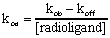
Analyzing competitive binding data

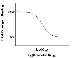
The top of the curve is a plateau at a value equal to radioligand binding in the absence of the competing unlabeled drug. This is total binding. The bottom of the curve is a plateau equal to nonspecific binding (NS). The difference between the top and bottom plateaus is the specific binding. Note that this not the same as B_max. When you use a low concentration of radioligand (to save money and avoid nonspecific binding), you have not reached saturation so specific binding will be much lower than the B_max.

The Y axis can be expressed as cpm or converted to more useful units like fmol bound per milligram protein or number of binding sites per cell. Some investigators like to normalize the data from 100% (no competitor) to 0% (nonspecific binding at maximal concentrations of competitor).

The concentration of unlabeled drug that results in radioligand binding halfway between the upper and lower plateaus is called the IC₅₀ (inhibitory concentration 50%) also called the EC₅₀ (effective concentration 50%). The IC₅₀ is the concentration of unlabeled drug that blocks half the specific binding.

If the labeled and unlabeled ligand compete for a single binding site, the steepness of the competitive binding curve is determined by the law of mass action. The curve descends from 90% specific binding to 10% specific binding with an 81-fold increase in the concentration of the unlabeled drug. More simply, nearly the entire curve will cover two log units (100-fold change in concentration).

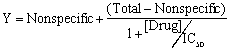
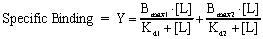
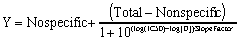
Competitive binding curves are described by this equation:

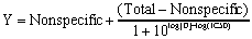
Y is the total binding you measure in the presence of various concentrations of the unlabeled drug, and log[D] is the logarithm of the concentration of competitor plotted on the X axis. Nonspecific is binding in the presence of a saturating concentration of D, and Total is the binding in the absence of competitor. Y, Total and Nonspecific are all expressed in the same units, such as cpm, fmol/mg, or sites/cell.

Use nonlinear regression to fit your competitive binding curve to determine the log(IC₅₀).

In order to determine the best-fit value of IC₅₀ (the concentration of unlabeled drug that blocks 50% of the specific binding of the radioligand), the nonlinear regression problem must be able to determine the 100% (total) and 0% (nonspecific) plateaus. If you have collected data over wide range of concentrations of unlabeled drug, the curve will have clearly defined bottom and top plateaus and the program should have no trouble fitting all three values (both plateaus and the IC₅₀).

With some experiments, the competition data may not define a clear bottom plateau. If you fit the data the usual way, the program might stop with an error message. Or it might find a nonsense value for the nonspecific plateau (it might even be negative). If the bottom plateau (0%) is incorrect, the IC₅₀ will also be incorrect. To solve this problem, you should define the nonspecific binding from other data. All drugs that bind to the same receptor should compete for all specific radioligand binding and reach the same bottom plateau value. When running the curve fitting program, set the bottom plateau of the curve to a constant equal to binding in the presence of a standard drug known to block all specific binding.

Similarly, if the curve doesn't have a clear top plateau, you should set the total binding to be a constant equal to binding in the absence of any competitor.

Calculating the K_i from the IC50

The value of the IC₅₀ is determined by three factors:

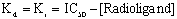
Calculate the K_i from the IC₅₀, using the equation of Cheng and Prusoff (Cheng Y., Prusoff W. H., Biochem. Pharmacol. 22: 3099-3108, 1973).

In thinking about this equation, remember that K_i is a property of the receptor and unlabeled drug, while IC₅₀ is a property of the experiment. By changing your experimental conditions (changing the radioligand used or changing its concentration), you'll change the IC₅₀ without affecting the K_i.

This equation is based on these assumptions:

Why determine log(IC₅₀) rather than IC₅₀?

The equation for a competitive binding curve (page 14) looks a bit strange since it combines logarithms and antilogarithms (10 to the power). A bit of algebra simplifies it :

If you fit the data to this equation, you'll get the same curve and the same IC₅₀. Since the equation is simpler, why not use it? The difference appears only when you look at how nonlinear regression programs assess the accuracy of the fit as a confidence interval. Even after converting from a log scale to a linear scale, you'll end up with different confidence intervals for the IC₅₀.

Which confidence interval is correct? With nonlinear regression, the standard error of the fit variables are only approximately correct. Since the confidence intervals are calculated from the standard errors, they too are only approximately correct. The problem is that the real confidence interval may not be symmetrical around the best fit value. It may extend further in one direction than the other. However, nonlinear regression programs always calculate symmetrical confidence intervals (unless you use advanced techniques). When writing the equation for nonlinear regression, therefore, you want to arrange the variables so the uncertainty is as symmetrical as possible. Because data are collected at concentrations of D equally spaced on a log axis, the uncertainty is symmetrical when the equation is written in terms of the log of IC₅₀, but is not symmetrical when written in terms of IC₅₀. You'll get more accurate confidence intervals from fits of competitive binding data when the equation is written in terms of the log(IC₅₀).

Homologous competitive binding curves

A competitive binding experiment is termed homologous when the same compound is used as the hot and cold ligand. The term heterologous is used when the hot and cold ligands differ. Homologous competitive binding experiments can be used to determine the affinity of a ligand for the receptor and the receptor number. In other words, the experiment has the same goals as a saturation binding curve. Because homologous competitive binding experiments use a single concentration of radioligand (which can be low), they consume less radioligand and thus are more practical when radioligands are expensive or difficult to synthesize.

To analyze a homologous competitive binding curve, you need to accept these assumptions:

Analyze a homologous competitive binding curve using the same equation used for a one-site heterologous competitive binding to determine the top and bottom plateaus and the IC₅₀.

The Cheng and Prussoff equation lets you calculate the K_i from the IC₅₀ (see page 15). In the case of a homologous competitive binding experiment, you assume that the hot and cold ligand have identical affinities so that K_d and K_i are the same. Knowing that, simple algebra converts the equation to:

You set the concentration of radioligand in the experimental design, and determine the IC₅₀ from nonlinear regression. The difference between the two is the K_d of the ligand (assuming hot and cold ligands bind the same).

The difference between the top and bottom plateaus of the curve represents the specific binding of radioligand at the concentration you used. Depending on how much radioligand you used, this value may be close to the B_max or far from it. To determine the B_max, divide the specific binding by the fractional occupancy, calculated from the K_d and the concentration of radioligand.

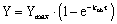
Kinetic binding experiments

What is a dissociation binding experiment?

A dissociation binding experiment measures the "off rate" for radioligand dissociating from the receptor. Perform dissociation experiments to:

To perform an off-rate experiment, first allow ligand and receptor to bind, perhaps to equilibrium. At that point, block further binding of radioligand to receptor using one of these methods:

After initiating dissociation, measure binding over time (typically 10-20 measurements) to determine how rapidly the ligand dissociates from the receptors.

How to analyze dissociation experiments

Fit the data to this equation using nonlinear regression to determine the rate constant. This is called an exponential decay equation.

Total binding and nonspecific binding (NS) are expressed in cpm, fmol/mg protein, or sites/cell. Time (t) is usually expressed in minutes. The dissociation rate constant (k_off) is expressed in units of inverse time, usually min^-1. Since it is hard to think in those units, it helps to calculate the half-life for dissociation which equals ln(2)/k_off or 0.6931/k_off. In one half-life, half the radioligand will have dissociated. In two half-lives, three quarters the radioligand will have dissociated, etc.

Typically the dissociation rate constant of useful radioligands is between 0.001 and 0.1 min^-1. If the dissociation rate constant is any faster, it would be difficult to perform radioligand binding experiments as the radioligand would dissociate from the receptors while you wash the filters.

Using a dissociation experiment to confirm the law of mass action

This analysis assumes that the law of mass action applies to your experimental situation. Dissociation binding experiments also let you test that assumption. If the law of mass action applies to your system, the answer to all these questions is yes:

Displaying dissociation data on a log plot

If you plot ln(specific binding) vs. time, the graph of a dissociation experiment will be linear if the system follows the law of mass action with a single affinity state. The slope of this line will equal -k_off.

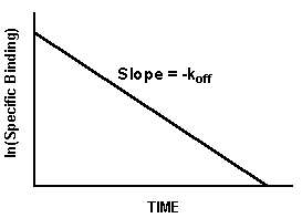
Notes:

• The log plot will only be linear if you take the logarithm of specific binding. A graph of log(total binding) vs. time will not be linear.
• You must use the natural logarithm, not the log base ten in order for the slope to equal -k_off.
• Use the log plot to display data, not to analyze data. You'll get a more accurate rate constant by fitting the raw data using nonlinear regression.

Association rate experiments

Association binding xperiments are used to determine the association rate constant. This is useful to characterize the interaction of the ligand with the receptor. It also is important as it lets you determine how long it takes to reach equilibrium in saturation and competition experiments.

You add radioligand and measure specific binding at various times thereafter.

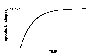
Note that the maximum binding (Y_max) is not the same as B_max. The maximum binding achieved in an association experiment depends on the concentration of radioligand. Low to moderate concentrations of radioligand will bind to only a small fraction of all the receptors no matter how long you wait.

To analyze the data, use nonlinear regression to fit the specific binding data to the one phase exponential association equation.

The observed rate constant, k_ob is expressed in units of inverse time, usually min^-1. It is a measure of how quickly the incubation reaches equilibrium, and is determined by three factors:

To calculate the association rate constant usually expressed in units of Molar^-1 min^-1, use the following equation. Typically ligands have association rate constants of about 10⁸ M^-1 min^-1.

Analyses of association experiments assume:

Combining association and dissociation data

Once you have separately determined k_on and k_off, you can combine them to calculate the K_d of receptor binding:

The units are consistent: k_off is in units of min^-1; k_on is in units of M^­1min^­1, so K_d is in units of M.

If binding follows the law of mass action, the K_d calculated this way should be the same as the K_d calculated from a saturation binding curve.

Two binding sites

Competitive binding with two sites

Competitive binding experiments are often used in systems where the tissue contains two classes of binding sites, perhaps two subtypes of a receptor. Analysis of these data are straightforward when you accept these assumptions:

If you accept those assumptions, binding follows this equation:

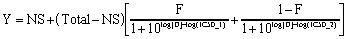
This equation has five variables: the total and nonspecific binding (the top and bottom binding plateaus), the fraction of binding to receptors of the first type of receptor (F), and the IC₅₀ of the unlabeled ligand for each type of receptors. If you know the K_d of the labeled ligand and its concentration, you can convert the IC₅₀ values to K_i values (see page 15).

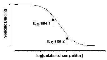
Since there are two different kinds of receptors with different affinities, you might expect to see a biphasic competitive binding curve. In fact, you will only see a biphasic curve only in unusual cases where the affinities are extremely different. More often you will see a shallow curve with the two components blurred together. For example, the following graph shows competition for two equally abundant sites with a ten fold (one log unit) difference in IC₅₀. If you look carefully, you can see that the curve is shallow (it takes more than two log units to go from 90% to 10% competition), but you cannot see two distinct components.

Analyzing saturation binding experiments with two sites

When the radioligand binds to two classes of receptors, analyze the data by using this equation.

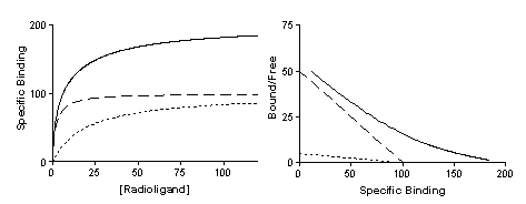
The left panel of the figure below shows specific binding to two classes of receptors present in equal quantities, whose K_d values differ tenfold. The right panel shows the transformation to a Scatchard plot. In both graphs the dotted and dashed lines show binding to the two individual receptors that sum to the solid curves.

Note the following:

Comparing one- and two-site models

A two-site model almost always fits your data better than a one-site model. A three-site model fits even better, and a four-site model better yet! As you add more variables (sites) to the equation, the curve becomes "more flexible" and gets closer to the points. You need to use statistical calculations to see if the improvement in fit between two-site and one-site models is more than you'd expect to see by chance.

Before thinking about statistical comparisons, you should look at whether the results make sense. Sometimes the two-site fit gives results that are clearly nonsense. Disregard a two-site fit when:

If the two-site fit seems reasonable, then you should test whether the improvement is statistically significant.

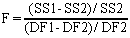
Even if the simpler one-site model is correct, you expect it to fit worse (have the higher sum-of-squares) because it has fewer inflection points (more degrees of freedom). In fact, statisticians have proven that the relative increase in the sum of squares (SS) is expected to equal the relative increase in degrees of freedom (DF). In other words, if the one-site model is correct you expect that:

If the more complicated two-site model is correct, then you expect the relative increase in sum-of-squares (going from two-sites to one-site) to be greater than the relative increase in degrees of freedom:

The F ratio quantifies the relationship between the relative increase in sum-of-squares and the relative increase in degrees of freedom.

If the one-site model is correct you expect to get an F ratio near 1.0. If the ratio is much greater than 1.0, there are two possibilities:

Many programs calculate the P value for you. If not, you can find it using a table of F statistics. You need to know that the numerator has DF1-DF2 degrees of freedom and the denominator has DF2 degrees of freedom. To use statistical tables you also have to remember that a larger value of F corresponds to a lower P value.

The P value answers this question: If the one-site model is really correct, what is the chance that you'd randomly obtain data that fits the two-site model so much better? If the P value is small, you conclude that the two-site model is significantly better than the one-site model. Most scientists reach this conclusion when P<0.05, but this threshold P value is arbitrary.

Advanced topics

The slope factor or Hill slope

Many competitive binding curves are shallower than predicted by the law of mass action for binding to a single site. The steepness of a binding curve can be quantified with a slope factor, often called a Hill slope. A one-site competitive binding curve that follows the law of mass action has a slope of -1.0. If the curve is more shallow, the slope factor will be a negative fraction (i.e. -0.85 or -0.60). The slope factor is negative because the curve goes downhill.

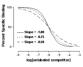
To quantify the steepness of a competitive binding curve (or a dose-response curve), fit the data to this equation:

The slope factor is a number that describes the steepness of the curve. In most situations, there is no way to interpret the value in terms of chemistry or biology. If the slope factor differs significantly from 1.0, then the binding does not follow the law of mass action with a single site.

Explanations for shallow binding curves include:

Agonist binding

All of the analyses presented in this booklet are based on the law of mass action. This assumes that the receptor and ligand reversibly bind, but nothing else happens. The law of mass action may not be true when the ligand or competitor is an agonist. By definition, something happens when an agonist binds to the receptor. For example, the agonist may alter the interaction of the receptor with a G protein, which then changes the affinity of the receptor for the agonist. These complexities mean that the law of mass action may be too simple when agonists are involved, and that the results of analyses based on the law of mass action can't be rigorously interpreted.

Some investigators have attempted to fit data to more complicated models, but these analyses are beyond the scope of this booklet. Despite the theoretical complexities, agonist binding curves often turn out to fit rectangular hyperbolas or one- or two-site competitive binding curves. Most investigators analyze their data using these standard analyses. The best-fit curves often fit the data nicely, and provide K_d or K_i values that can be compared between conditions. It is important to realize that these analyses are based on a model that is too simplistic. Treat the best-fit values of K_d or K_i as empirical descriptions of the data, and are not as true equilibrium dissociation constants.

Ligand depletion

The equations that describe the law of mass action include the variable [Ligand] which is the free concentration of ligand. All the analyses presented so far depend on the assumption that a very small fraction of the ligand binds to receptors (or to nonspecific sites) so you can assume that the free concentration of ligand is approximately equal to the concentration added. This is sometimes called "zone A".

In some experimental situations, the receptors are present in high concentration and have a high affinity for the ligand, so that assumption is not valid. A large fraction of the radioligand binds to receptors so the free concentration of radioligand is quite a bit lower than the concentration added. The system is not in "zone A". The discrepancy is not the same in all tubes or at all times.

Many investigators use this rule of thumb. If less than 10% of the ligand binds, don't worry about ligand depletion.

If possible you should design your experimental protocol to avoid situations where more than 10% of the ligand binds. You can do this by using less tissue in your assays. The problem is that this will also decrease the number of counts. An alternative is to increase the volume of the assay without changing the amount of tissue. The problem with this approach is that you'll need more radioligand.

If you can't avoid radioligand depletion, you need to account for the depletion in your analyses. You may use several approaches.

GraphPad Prism

All the graphs in this booklet were created using GraphPad Prism, a general-purpose curve fitting and scientific graphics program for Windows.

Although GraphPad Prism was designed to be a general purpose program, it is particularly well-suited for analyses of radioligand binding data.

Please visit our web site at http://www.graphpad.com to read about Prism and download a free demo. Or contact GraphPad Software to request a brochure and demo disk by phone (619-457-3909), fax (619-457-8141) or email sales@graphpad.com. The demo is not a slide show - it is a functional version of Prism with no limitations in data analysis. Try it out with your own data, and see for yourself why Prism is the best solution for analyzing and graphing scientific data.

Back to the Pharmacology Guide